Persisting and running machine learning models with ONNX

We often train machine learning models on one machine and predict from them on another later. This creates the need to persist the trained model, which raises the question of finding the most suitable serialization format. The scikit-learn team strongly recommends ONNX in their documentation if the persisted model is only used for inference later.

This post is the first in a series of three on ONNX in general and the tools we built to integrate it into our projects. In this installment, we explore in detail what "persisting a model" actually means and how ONNX is a tool designed precisely for the set requirements. The second post focuses on efficiently defining ONNX graphs using an open-source library developed here at QuantCo named Spox. Lastly, we will glimpse into the bright and imminent future promised by the array API and our ONNX-backed implementation of it, ndonnx.

Persisting a machine learning model

Let us consider a typical scikit-learn-like model¹ and how one may persist an instance of it:

# model.py

from scipy import linalg
import numpy as np

class LinearRegression:
    def fit(self, X, y):
        y_offset = np.average(y, axis=0)
        X_offset = np.average(X, axis=0)
        self._coefficients, *_ = linalg.lstsq(X - X_offset, y - y_offset)
        self._intercept = y_offset - X_offset @ self._coefficients

    def predict(self, X):
        return X @ self._coefficients + self._intercept

Calling fit() on a LinearRegression instance sets the state of the _coefficients and _intercept fields. The predict() function encapsulates the inference logic and relies on the trained values. A common approach to persist an instance of LinearRegression is to use Python's built-in pickle module:

import pickle

import numpy as np

X = np.array([[0, 0], [1, 1], [2, 2]], np.float32)
y = np.array([1, 2, 3], np.float32)

model = LinearRegression()
model.fit(X, y)

with open("model.pkl", "wb") as f:
    pickle.dump(model, f)
    

However, there is a catch (or rather several): Pickle files only contain the state of objects, but not the implementation logic that is needed to do anything useful with the objects they contain. The production environment where we want to use our trained model must provide a LinearRegression class compatible with the pickled data, and sometimes this is hard to ensure. To understand this issue, let us consider that after creating a model.pkl file, we renamed the private field self._coefficients to self._weights.

import pickle

import numpy as np


class LinearRegression:
    def fit(self, X, y):
        ...

    def predict(self, X):
        # Renamed `self._coefficients` to `self._weights`
        return X @ self._weights + self._intercept


with open("model.pkl", "rb") as f:
    model = pickle.load(f)
    

This seemingly inconspicuous change already did the trick. The pickle library is, understandably, unable to map the older serialized state to the new class definition, leaving self._weights undefined after the deserialization. This, in turn, creates the following exception at inference:

X = np.array([[0, 0], [1, 1], [2, 2]])
model.predict(X)

>>> AttributeError: 'LinearRegression' object has no attribute '_weights'

One may strive to avoid this issue in self-maintained code, but this is impossible for third-party dependencies. While there are ways to salvage the situation, real-world cases may quickly become far more complex than the one presented here.

Abstractly, the trouble originates from the serialized state becoming incompatible with the latest version of the model's predict implementation. Ideally, we would like to persist a copy of the inference code and all its dependencies inside the pickle file, too. However, pickle is not designed for such a task. While we may not be able to include the code inside a pickle file, we may bundle the entire training environment with it. One way to create such a bundle is to persist the environment and pickle file in a Docker image, but this severely complicates how a model may be used. A more flexible solution is to pin every dependency (including transitive ones) to the version used during training and then enforce these pins using a package manager. However, this creates a whole new set of issues. The most obvious problem arises if the dependency constraints in the production environment are not solvable under the required pins. If they are solvable, the pinning may still introduce security vulnerabilities, the inability to load various models trained at different points in time in a single Python process, or the simple fact that the production environment gets bloated by training-related dependencies (such as SciPy in the given example).

Fortunately, there is a better way!

Describing a model as a self-contained computational graph

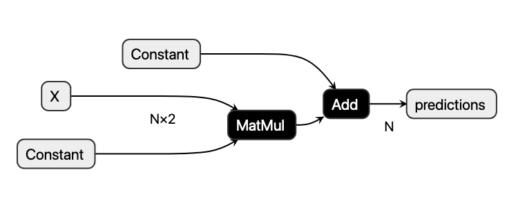
If one examines the inference logic in LinearRegression.predict, one may realize that it consists of a chain of pure tensor transformations. This observation applies to most machine learning models. Furthermore, we may interpret the chain of tensor operations as a computational acyclic graph that may be visualized as follows:

The node shapes denote different types of nodes. Rectangular shapes represent inputs and outputs, while hexagons mark constant tensors. Boxes with rounded corners denote operations that take input tensors and produce output tensors in turn.

One may quickly invent a JSON-based format that describes the above inference logic and contains the state of the discussed model instance:

{
    "inputs": ["X"],
    "outputs": ["predictions"],
    "constants": {
        "coefficients": [0.5, 0.5],
        "intercept": [1.0]
    },
    "computational_graph": [
        {
            "operation": "MatMul",
            "inputs": ["X", "coefficients"],
            "outputs": ["matmul_result"]
        },
        {
            "operation": "Add",
            "inputs": ["matmul_result", "intercept"],
            "outputs": ["predictions"]
        }
    ]
}

Let us ignore for a moment that JSON is a terrible format for serializing numerical data² and that there is no efficient way to create such JSON data from a model instance in the first place. Instead, we assume that the above JSON snippet is stored in a file named model.json. How may one use such a file to compute a prediction?

While JSON is not directly executable, one may write a crude inference engine that interprets the computational graph. Such an engine needs to read the provided JSON file, set up the constants as NumPy arrays, and provide a function that takes input tensors and returns the desired predictions:

import json

import numpy as np


class InferenceEngine:
    """Very crude inference engine for our custom serialization format."""
    
    def __init__(self, path):
        with open(path) as f:
            self._model_dict = json.load(f)

        self._constants = {}
        for name, const in self._model_dict["constants"].items():
            self._constants[name] = np.array(const)


    def infer(self, **inputs: np.ndarray) -> dict[str, np.ndarray]:
        scope = inputs | self._constants
        
        # We assume that the operations are in topological order
        for op_dict in self._model_dict["computational_graph"]:
            op_inputs = [scope[name] for name in op_dict["inputs"]]
            op_name = op_dict["operation"]
            if op_name == "MatMul":
                output_name, = op_dict["outputs"]
                scope[output_name] = np.matmul(*op_inputs)
            elif op_name == "Add":
                output_name, = op_dict["outputs"]
                scope[output_name] = np.add(*op_inputs)                
            else:
                raise NotImplementedError(f"Operation `{op_name}` is not implemented.")

        return {name: value for name, value in scope.items() if name in self._model_dict["outputs"]}

With such an inference engine at hand, we are now able to perform predictions in a way that is completely independent of our training environment:

engine = InferenceEngine("model.json")

X = np.array([[0, 0], [1, 1], [2, 2]], np.float32)
engine.infer(X=X)

>>> {'predictions': array([1., 2., 3.])}

A more advanced inference engine may utilize specialized hardware, such as GPUs, for operations that benefit from it. Furthermore, one may write the engine in a compiled language such as Rust or C++, which opens interesting possibilities. Firstly, a compiled engine will likely yield better performance and multi-threading opportunities than one written in Python. Secondly, such an engine would also enable deploying models trained in Python in scenarios where Python is unavailable or unfeasible such as on mobile devices or in the browser.

However, by hand-rolling our own serialization format, we have frankly created many new problems, too:

• The serialization format and the operator semantics must be backward compatible and well-specified to allow old models to be used with our engine's latest version. Even for operators as simple as the ones used in the above example, one would have to define their type promotion rules and broadcasting behavior meticulously.
• Developing and maintaining a complex high-performance inference engine requires considerable resources.
• We have to solve the question of serializing our trained model into whatever format we choose.

We will leave the last point for the next two posts in this series. For now, we are content to recognize that the first two points are easy to solve: Rather than reinventing the wheel, we use existing and well-established open-source tools. Chiefly at our disposal are the publicly available ONNX specification and the inference engine built on top of it, aptly named onnxruntime.

As luck (or premonition of the author) would have it, ONNX follows just the same design logic as the custom JSON format laid out above: On one hand, the ONNX project specifies around 200 standard operations. Among these are operators such as the Add and MatMul as one may expect, but also much more sophisticated ones defining convolutions or boosted decision trees. On the other hand, ONNX defines a file format for the computational graph that is very similar to the JSON schema derived above, but rather than JSON, it is based on protobuf. The exact details of the schema can be found upstream. However, as we will discover in the next part of this series, users should virtually never find themselves interacting with ONNX on such a low level.

Nonetheless, here is the ONNX counterpart of the model.json defined in protobuf via the official onnx Python package:

import onnx
from onnx import helper as oh

onnx_model = oh.make_model(
    oh.make_graph(
        name="graph",
        inputs=[oh.make_tensor_value_info("X", oh.TensorProto.FLOAT, ("N",2 ))],
        outputs=[oh.make_tensor_value_info("predictions", oh.TensorProto.FLOAT, ("N",))],
        nodes=[
            oh.make_node("Constant", inputs=[], outputs=["coefficients"], value_float=[0.5, 0.5]),
            oh.make_node("Constant", inputs=[], outputs=["intercept"], value_float=1.0),
            oh.make_node("MatMul", inputs=["X", "coefficients"], outputs=["matmul_result"]),
            oh.make_node("Add", inputs=["matmul_result", "intercept"], outputs=["predictions"])
        ]
    ),
    ir_version=8
)

onnx.save(onnx_model, "model.onnx")

We set an explicit ir_version that governs details of the produced protobuf layout to ensure compatibility with the current onnxruntime release. The last line wrote the onnx_model protobuf object to the model.onnx file. The API is largely self-describing and hints that ONNX does offer more features than the above JSON format. An ONNX model consists of a graph and possibly further metadata. The graph's inputs and outputs are named, strongly typed, and of static rank. The length of a dimension may be defined using a placeholder such as "N" that will be determined at inference time or as a constant. The inputs and outputs of each node are referenced by name. Notably, intermediate values such as "matmul_result" do not require an explicit type and shape annotation.

We may also visualize the model stored in model.onnx using netron.app:

Analogously to the use of the InferenceEngine with our JSON file, we may create an onnxruntime.InferenceSession from the model.onnx file:

import onnxruntime as ort


session = ort.InferenceSession("model.onnx")

Once instantiated, the session offers a way to run inference on the model as expected:

session.run(input_feed={"X": X}, output_names=["predictions"])

>>> [array([1., 2., 3.], dtype=float32)]

This demonstrates that ONNX is a feasible serialization format for trained models and that we may use it to predict from models without pining any training dependencies. However, the elephant in the room remains: How can one convert a trained Python model into an ONNX model in a convenient and scalable way? This question is answered in parts two and three of this series.